개발/💠 Alchemist
💠 분류 - 캐글 산탄데르 고객 만족 예측 💠
정소은
2023. 10. 31. 18:37
< 캐글 산탄데르 고객 만족 예측 >
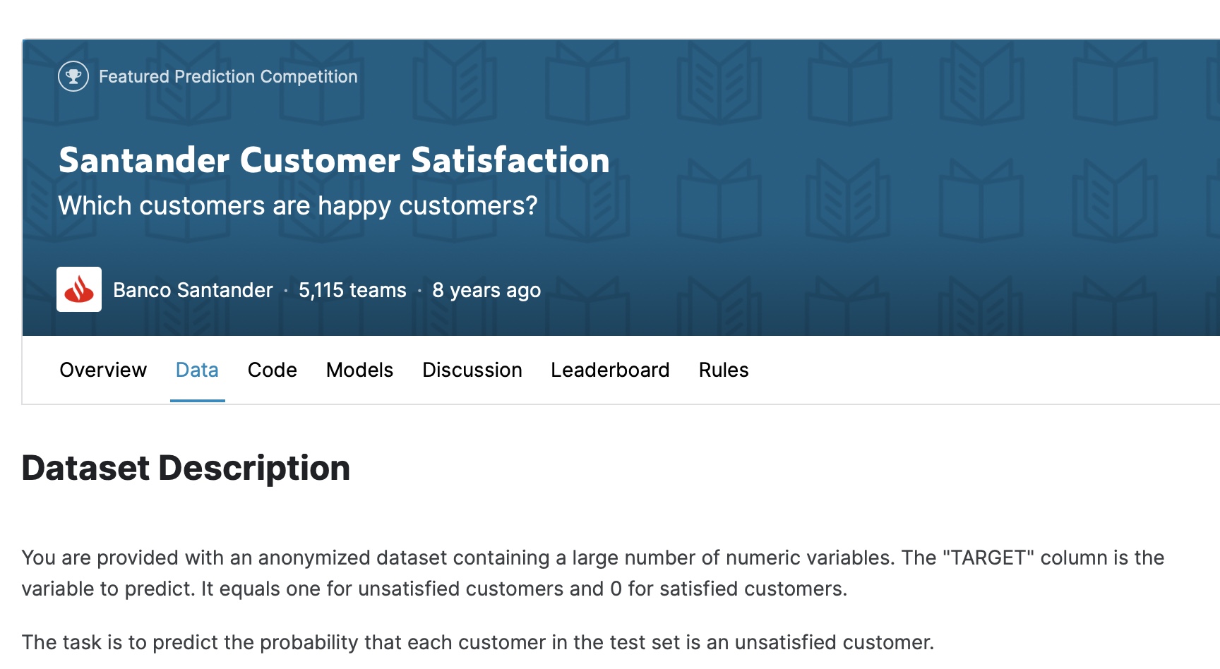
1. 데이터세트 로딩 및 데이터 세트 전처리
패키지, dataset import
import numpy as np
import pandas as pd
import matplotlib.pyplot as plt
import matplotlib
import warnings

warnings.filterwarnings('ignore')
cust_df = pd.read_csv('/Users/jeongsoeun/Downloads/train.csv', encoding='latin-1')

# 데이터세트 행렬 파악 : (76020, 371)
print('dataset shape:', cust_df.shape)

# 데이터세트 3줄 출력
cust_df.head(3)
dataset 정보 파악 - feature 371개 존재
cust_df.info()
피처의 레이블 정보 파악
print(cust_df['TARGET'].value_counts())
unsatisfied_cnt = cust_df[cust_df['TARGET']==1].TARGET.count()
total_cnt = cust_df.TARGET.count()
print('unsatisfied 비율은 {0:.2f}'.format((unsatisfied_cnt / total_cnt)))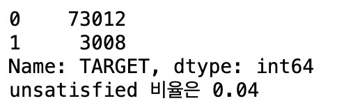
모두 숫자형이며 float형 111개, int형 260개, Null값은 없음
'Target' 칼럼 - 대부분이 만족이고 불만족이 4%에 불과한 불균형한 레이블값을 가짐
피처값의 분포 확인
cust_df.describe()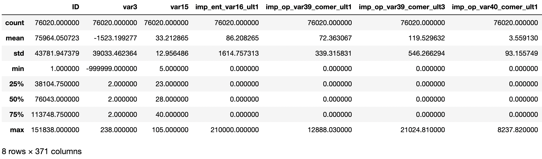
'var3' 칼럼 - min값이 -999999 / -999999 값이 116개 존재 (다른 값에 비해 편차가 심하기 때문에 모델 성능에 나쁜 영향을 줌)
dataset 조정
# -999999값을 가장 값이 많은 2로 변환
cust_df['var3'].replace(-999999,2,inplace=True)

# 무의미한 'ID' 칼럼 drop
cust_df.drop('ID', axis=1, inplace=True)

# 피처 세트와 레이블 세트 분리
X_features = cust_df.iloc[:, :-1]
y_labels = cust_df.iloc[:, -1]
print('피처 데이터 shape:{0}'.format(X_features.shape))
2. 학습 / 테스트 데이터 분리
학습 / 테스트 데이터 분리
from sklearn.model_selection import train_test_split

# 학습/테스트 데이터 분리
X_train, X_test, y_train, y_test = train_test_split(X_features, y_labels, test_size=0.2, random_state=0)

# 학습/테스트 데이터의 Target의 학습/테스트 세트 레이블값 분포 확인
train_cnt = y_train.count()
test_cnt = y_test.count()

print('학습 세트 Shape:{0}, 테스트 세트 Shape:{1}'.format(X_train.shape, X_test.shape))
print('학습 세트 레이블 값 분포 비율')
print(y_train.value_counts()/train_cnt)
print('\n테스트 세트 레이블 값 분포 비율')
print(y_test.value_counts()/test_cnt)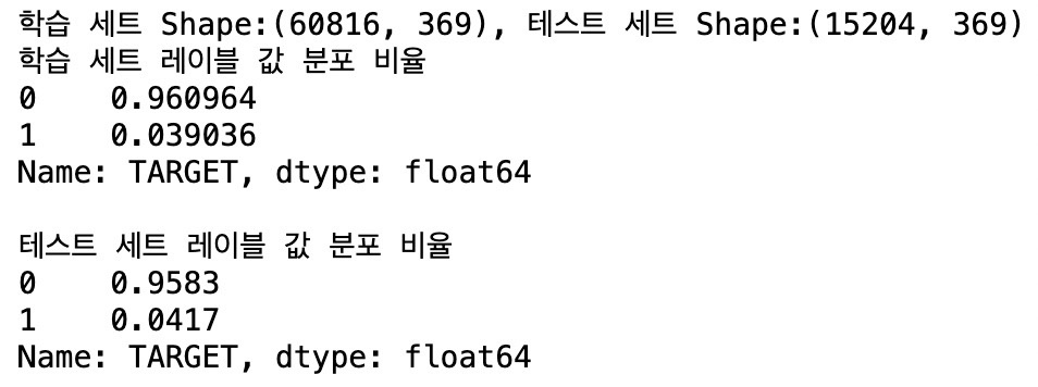
학습 세트 - 학습 / 검증 세트로 분리
X_tr, X_val, y_tr, y_val = train_test_split(X_train, y_train, test_size = 0.3, random_state = 0)
< XGBClassifier 이용 >
3. XGBClassifier의 하이퍼 파라미터 튜닝
XGBoost 모델 학습과 하이퍼 파라미터 튜닝
from xgboost import XGBClassifier
from sklearn.metrics import roc_auc_score

# XGBClassifier 객체 생성
xgb_clf = XGBClassifier(n_estimators=500, learning_rate=0.05, random_state=156)

# XGBClassifier 모델 학습
xgb_clf.fit(X_tr, y_tr, early_stopping_rounds=100, eval_metric="auc", eval_set=[(X_tr, y_tr),(X_val, y_val)])

# XGBClassifier 성능 평가 - ROC AUC -> 결과 : 0.8429
xgb_roc_score = roc_auc_score(y_test, xgb_clf.predict_proba(X_test)[:,-1])
print('ROC AUC: {0:.4f}'.format(xgb_roc_score))
XGBoost 하이퍼 파라미터 튜닝 - HyperOpt
from hyperopt import hp

## 검색 공간 설정 ##
# max_depth는 5~15까지 1 간격으로, min_child_weight는 1~6까지 1 간격으로
# colsample_bytree는 0.5~0.95 사이, learning_rate는 0.01~2 사이 정규 분포된 값으로 검색공간 설정
xgb_search_space = {'max_depth':hp.quniform('max_depth',5,15,1),
                   'min_child_weight':hp.quniform('min_child_weight',1,6,1),
                   'colsample_bytree':hp.uniform('colsample_bytree',0.5,0.95),
                   'learning_rate':hp.uniform('learning_rate',0.01,0.2)}
## 목적 함수 생성 ##

from sklearn.model_selection import KFold
from sklearn.metrics import roc_auc_score


# fmin()에서 호출 시 search_space 값으로 XGBClassifier 교차 검증 학습 후 -1*roc_auc 평균 값 반환
def objective_func(search_space):
	# XGBoost 객체 생성
    xgb_clf = XGBClassifier(n_estimators = 100, max_depth = int(search_space['max_depth']),
                           min_child_weight = int(search_space['min_child_weight']),
                           colsample_bytree = search_space['colsample_bytree'],
                           learning_rate = search_space['learning_rate'])

    # 3개 k-fold 방식으로 평가된 roc_auc 지표를 담는 list
    roc_auc_list = []

    # 3개 k-fold 방식 적용
    kf = KFold(n_splits=3)
    # X_train을 다시 학습과 검증용 데이터로 분리
    for tr_index, val_index in kf.split(X_train):
        X_tr, y_tr = X_train.iloc[tr_index], y_train.iloc[tr_index]
        X_val, y_val = X_train.iloc[val_index], y_train.iloc[val_index]

        # early stopping은 30회로 설정하고 추출된 학습과 검증 데이터로 XGBClassifier 학습 수행
        xgb_clf.fit(X_tr, y_tr, early_stopping_rounds=30, eval_metric="auc",
                    eval_set = [(X_tr, y_tr),(X_val, y_val)])

        # 1로 예측한 확률값 추출 후 roc auc 계산을 위해 list에 결괏값 담음
        score = roc_auc_score(y_val, xgb_clf.predict_proba(X_val)[:, 1])
        roc_auc_list.append(score)

    # 3개 k-fold로 계산된 roc_auc 값의 평균값을 반환하되
    # HyperOpt는 목적함수의 최솟값을 위한 입력값을 찾으므로 -1 곱한 뒤 반환
    return -1*np.mean(roc_auc_list)
## 최적 하이퍼 파라미터 도출 ##

from hyperopt import fmin, tpe, Trials

trials = Trials()

# fmin() 함수 호출, max_evals 지정된 횟수(50)만큼 반복 후 목적함수의 최솟값을 가지는 최적 입력값 추출
best = fmin(fn=objective_func,
           space=xgb_search_space,
           algo=tpe.suggest,
           max_evals=50,
           trials=trials, rstate=np.random.default_rng(seed=30))

print('best:',best)
결과 - colsample_bytree : 0.5749, learning_rate : 0.1514, max_depth : 5.0, min_child_weight : 6.0
4. XGBClassifier 적용
최적 하이퍼 파라미터 값으로 XGBClassifier 재학습
# XGBClassifier 객체 생성
xgb_clf = XGBClassifier(n_estimators=500, learning_rate=round(best['learning_rate'], 5),
                       max_depth=int(best['max_depth']),
                       min_child_weight=int(best['min_child_weight']),
                       colsample_bytree=round(best['colsample_bytree'], 5))

# 모델 학습
xgb_clf.fit(X_tr, y_tr, early_stopping_rounds=100,
           eval_metric="auc", eval_set=[(X_tr, y_tr),(X_val, y_val)])

# 모델 예측 성능 평가
xgb_roc_score=roc_auc_score(y_test, xgb_clf.predict_proba(X_test)[:,1])
print('ROC AUC: {0:.4f}'.format(xgb_roc_score))
결과 - ROC AUC 값 : 0.8457 ( 하이퍼 파라미터 튜닝 전보다 성능 상승 )
feature 중요도 그래프
from xgboost import plot_importance
import matplotlib.pyplot as plt
%matplotlib inline

fig, ax = plt.subplots(1,1,figsize=(10,8))
plot_importance(xgb_clf, ax=ax, max_num_features=20, height=0.4)
< Light GBM 이용 >
4. LGBMClassifier
LGBMClassifier 학습과 하이퍼 파라미터 튜닝
from lightgbm import LGBMClassifier

# LGBMClassifier 객체 생성
lgbm_clf = LGBMClassifier(n_estimators=500)

# 학습/검증 데이터세트
eval_set = [(X_tr, y_tr),(X_val, y_val)]

# 모델 학습
lgbm_clf.fit(X_tr, y_tr, early_stopping_rounds=100, eval_metric="auc", eval_set = eval_set)

# 모델 성능 평가 - roc_auc
lgbm_roc_score = roc_auc_score(y_test, lgbm_clf.predict_proba(X_test)[:,1])
print('ROC AUC: {0:.4f}'.format(lgbm_roc_score))
5. LGBMClassifier 하이퍼 파라미터 튜닝 - HyperOpt
# LGBMClassifier 검색 공간 설정

lgbm_search_space = {'num_leaves':hp.quniform('num_leaves',32,64,1),
                    'max_depth':hp.quniform('max_depth',100,160,1),
                    'min_child_samples':hp.quniform('min_child_samples',60,100,1),
                    'subsample':hp.uniform('subsample', 0.7, 1),
                    'learning_rate':hp.uniform('learning_rate',0.01, 0.2)}
# 목적 함수 생성

def objective_func(search_space):
    lgbm_clf = LGBMClassifier(n_estimator=100,
                             num_leaves=int(search_space['num_leaves']),
                             max_depth=int(search_space['max_depth']),
                             min_child_samples=int(search_space['min_child_samples']),
                             subsample=search_space['subsample'],
                             learning_rate= search_space['learning_rate'])

    roc_auc_list = []

    kf = KFold(n_splits=3)

    for tr_index, val_index in kf.split(X_train):
        X_tr, y_tr = X_train.iloc[tr_index], y_train.iloc[tr_index]
        X_val, y_val = X_train.iloc[val_index], y_train.iloc[val_index]

        lgbm_clf.fit(X_tr, y_tr, early_stopping_rounds = 30, eval_metric = "auc",
                    eval_set = [(X_tr, y_tr),(X_val, y_val)])

        score = roc_auc_score(y_val, lgbm_clf.predict_proba(X_val)[:, 1])
        roc_auc_list.append(score)

    return -1*np.mean(roc_auc_list)
# 최적 하이퍼 파라미터 도출
from hyperopt import fmin, tpe, Trials

trials = Trials()

best = fmin(fn=objective_func, space=lgbm_search_space, algo=tpe.suggest, max_evals=50, trials=trials, rstate=np.random.default_rng(seed=30))

print('best:',best)
결괏값 - learning_rate : 0.08592, max_depth : 121.0, min_child_samples : 69.0, num_leaves : 41.0, subsample : 0.91489
5. LGBMClassifier 적용
LGBMClassifier 적용
lgbm_clf = LGBMClassifier(n_estimators=500, num_leaves=int(best['num_leaves']),
                         max_depth=int(best['max_depth']),
                         min_child_samples=int(best['min_child_samples']),
                         subsample=round(best['subsample'], 5),
                         learning_rate=round(best['learning_rate'],5))

lgbm_clf.fit(X_tr, y_tr, early_stopping_rounds=100,
            eval_metric="auc", eval_set=[(X_tr, y_tr),(X_val, y_val)])

lgbm_roc_score = roc_auc_score(y_test, xgb_clf.predict_proba(X_test)[:,1])
print('ROC AUC: {0:.4f}'.format(lgbm_roc_score))